Adaptive early termination for HNSW in Elasticsearch

From vector search to powerful REST APIs, Elasticsearch offers developers the most extensive search toolkit. Dive into our sample notebooks in the Elasticsearch Labs repo to try something new. You can also start your free trial or run Elasticsearch locally today.

Elasticsearch uses the Hierarchical Navigable Small World (HNSW) algorithm to perform vector search over a proximity graph. HNSW is known to provide a nice trade-off between the quality of k-nearest neighbor (KNN) results and the associated cost.

In HNSW, search proceeds by iteratively expanding candidate nodes in the graph, maintaining a bounded set of nearest neighbors discovered so far. Each expansion has a cost (vector operations, random seeks to disk, and more), and the marginal benefit of that cost tends to decrease as the search progresses.

One way to optimize HNSW graph traversal is to stop searching when the marginal likelihood of finding new true neighbors doesn’t increase. For this reason, in Elasticsearch 9.2 we introduced a new early termination mechanism. This stops the search process when visiting graph nodes doesn’t provide enough new nearest neighbors, consecutively, for a fixed number of times.

This article guides you through how we improved over the mentioned early termination mechanism in HNSW to make it better suited for different datasets and data distributions.

Early termination in HNSW

In HNSW, search proceeds by iteratively expanding candidate nodes in the proximity graph, maintaining a bounded set of nearest neighbors discovered so far, until it either has visited the whole graph or meets some early stop criteria.

Early termination is therefore not necessarily always an optimization, it’s part of the search algorithm itself. The moment we decide to stop determines the balance between efficiency and recall. In Elasticsearch, there are already a number of ways a query on HNSW can early terminate:

• A fixed maximum number of nodes is visited.
• A fixed timeout is reached.

While simple and predictable, these rules are largely agnostic to what the search is actually doing. Also they’re used mostly to make sure that the query finishes in reasonable time for the end user.

In a previous blogpost, we introduced the concept of redundancy in HNSW. In short, redundant computations occur when HNSW continues to evaluate new candidate nodes that don’t result in finding more nearest neighbors.

Patience: Measuring progress instead of effort

The notion of patience reframes early termination around progress rather than effort.

Instead of asking:

“How many steps have we taken?”

The new question becomes:

“What is the amount of computation we accept to waste, until we lose hope?”

During HNSW search, early exploration typically produces peak improvements to the top-k candidate set. During first steps of the HNSW graph exploration, the set of neighbors is continuously updated as the algorithm keeps discovering nearer and nearer neighbors to the query vector. Over time, these improvements become rarer as the search converges. Patience-based termination monitors this pattern and terminates the search once improvements have ceased for a sustained period.

In practice, while visiting the HNSW graph we also compute the queue saturation ratio as we hop through candidate nodes. This measures the percentage of nearest neighbors that were left unchanged while visiting the most recent graph node (or the inverse of the number of new neighbors introduced during the last iteration). When such a ratio becomes too big for too many consecutive iterations, we stop visiting the graph.

Conceptually, patience treats HNSW search as a diminishing returns process. When returns flatten out, continuing to explore the graph yields little benefit.

This framing is powerful because it ties termination directly to observable outcomes rather than to arbitrary fixed limits.

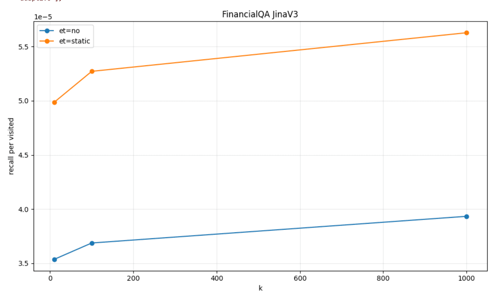
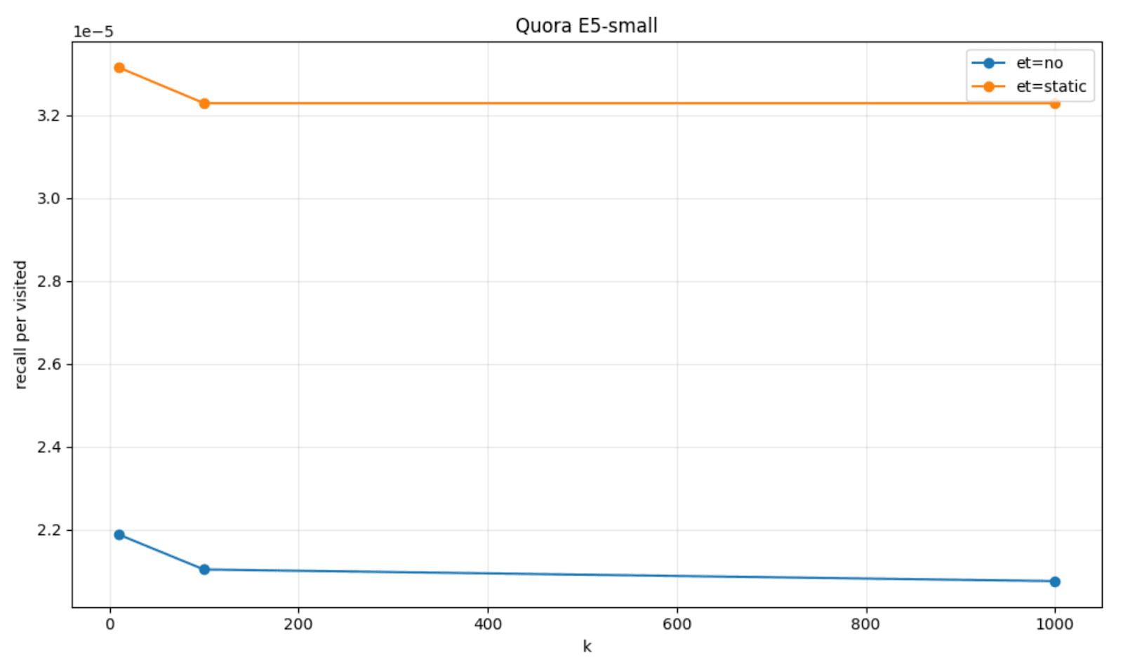
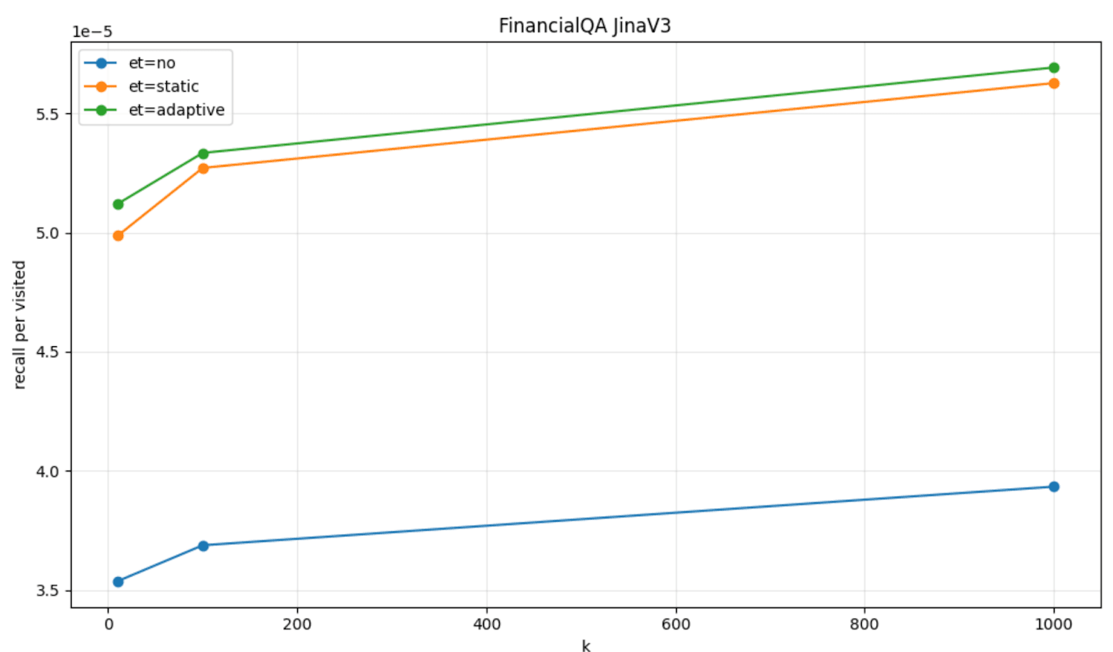
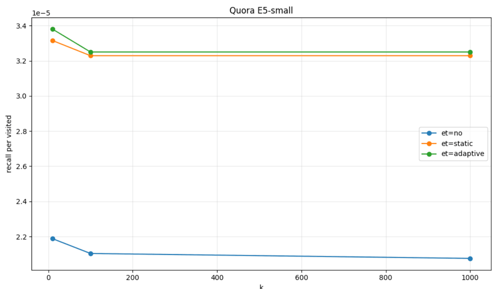
The benefit of using this smart early termination technique is that HNSW graph explorations tend to visit a smaller number of graph nodes while retaining an almost perfect relative recall.

To visualize this, we can plot the amount of recall per visited node that we got with the patience based early termination (labeled as et=static), when compared to the default HNSW behavior (labeled as et=no) on a couple of datasets, FinancialQA and Quora, and models, JinaV3 and E5-small.

Static thresholds and HNSW dynamics

In practice, in Elasticsearch this is implemented using static thresholds. One threshold refers to the saturation threshold: that is, the ratio of saturation that we consider suboptimal. The other threshold refers to the number of consecutive graph nodes that we allow to be visited while still having a suboptimal queue saturation: that is, the patience threshold.

When we introduced this early termination strategy in Elasticsearch 9.2, we decided to opt for conservative defaults, so as to let the recall as much as possible, while still gaining in terms of latency and memory consumption. For this reason, we set the saturation threshold to be 100% and the patience threshold to be set as a (bounded) 30% of the num_candidates in the KNN query.

In many scenarios, these settings resulted to work nicely; however, two queries requesting the same number of neighbors might have radically different convergence behaviors. Some queries encounter dense local neighborhoods and saturate quickly; others must traverse long, sparse paths before finding competitive candidates. The latter resulted to be the most difficult to handle effectively.

As a result, we sometimes noticed:

• Over-exploration for easy queries.
• Premature termination for hard queries.

Therefore, we figured that fixed threshold values encode global assumptions about convergence, whereas we could make HNSW better adapt to different dynamics.

Making HNSW early termination adaptive

Adaptive early termination approaches this problem from a different angle. Instead of enforcing predefined stopping thresholds, the algorithm infers when to stop from the search dynamics themselves.

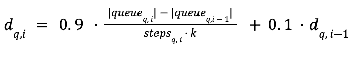
So instead of comparing the queue saturation ratio between two consecutive candidates, we decided to introduce both an instant smoothed discovery rate $d_{q,i}$ (how many new neighbors were introduced for a query q, in the last visit i) together with rolling mean $\mu_{q,i}$ and standard deviation $\sigma_{q,i}$ of such a discovery rate during the graph visit (using Welford’s algorithm). These statistics about the discovery rate are calculated per query, so that this information can be used to decide different degrees of patience for each query.

The previously static thresholds become adaptive to the discovery rate statistics: The saturation threshold becomes the rolling mean plus the standard deviation; whereas we make the patience adapt and scale inversely with the standard deviation.

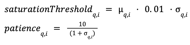
The early exit rules remain the same; the saturation happens when the instant discovery rate is lower than the adaptive saturation threshold. The graph visit stops if the saturation persists for a number of consecutive candidate visits that’s larger than the adaptive patience.

This way, we obtain a behavior that doesn’t depend on the num_candidates parameter in the KNN query (which might be always set or left as the default, regardless of early exit) and that better adapts to each query and vector distribution dynamically.

The recall per visited node on FinancialQA and Quora with the adaptive strategy (labeled as et=adaptive) reports a higher recall per visited node, when compared to the static strategy (et=static) and the default HNSW behavior (et=no).

Adaptive early termination is turned on by default in Elasticsearch 9.3 for HNSW dense vector fields (and it can eventually be turned off via the same index level setting).