HNSW graph: How to improve Elasticsearch performance

New to Elasticsearch? Join our getting started with Elasticsearch webinar. You can also start a free cloud trial or try Elastic on your machine now.

The principles of Hierarchical Navigable Small World vector searches were first introduced in Elasticsearch 8.0. But how are graphs created in the first place? What effect does graph construction have on search quality? And what do those parameters actually do?

Searching the graph

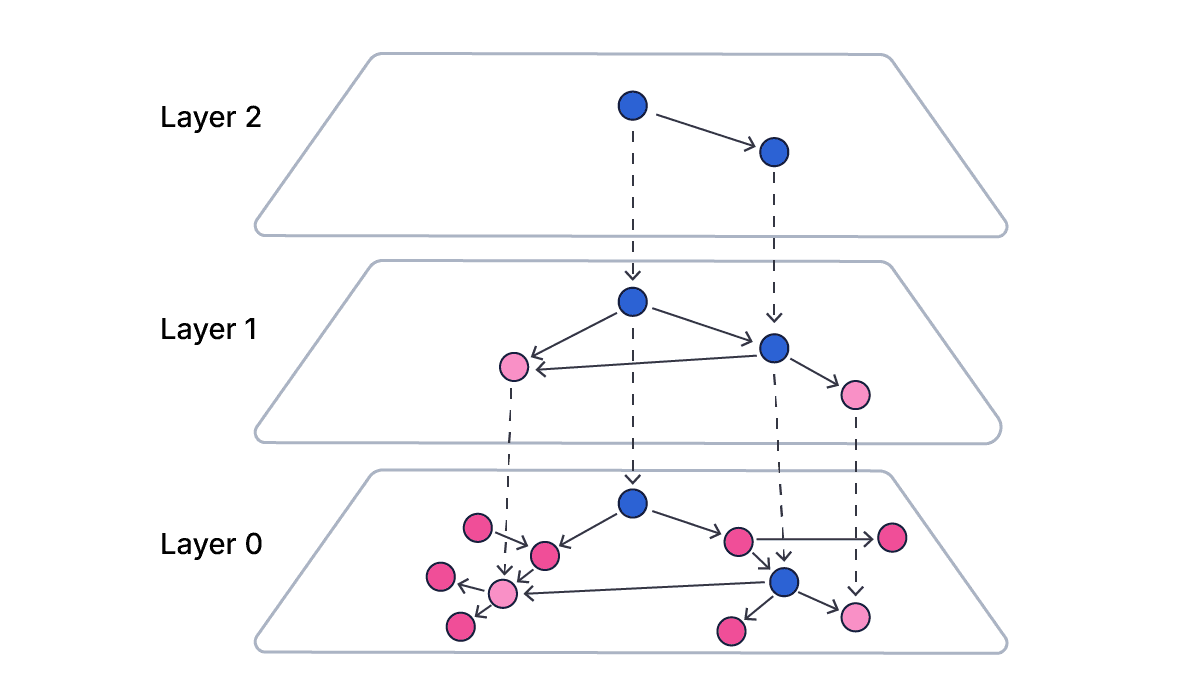
To start with, a brief recap of how HNSW graphs work. An HNSW graph is a layered data structure, with the following rules:

All vectors are present in the bottom layer (layer 0); each vector is represented by a graph node in that layer.
The probability of a vector appearing in each layer decreases logarithmically as you go up the layers, so each layer will have fewer vectors than the layer below it.
Each vector present in a layer is represented by a node in that layer. All the nodes for the same vector are associated with that vector.
If a vector is present in a layer, it will also be present in all lower layers, down to layer 0
Each node on each layer has references to a certain number of other nodes on the same layer, generally the closest nodes (as determined by the vector similarity, see below).
References are one-directional, so if node A references node B, node B does not necessarily reference node A.

Each segment of a Lucene index has its own independent HNSW graph, containing just the vectors in that segment. Multiple segments are searched independently.

An HNSW graph works no matter the number of dimensions of the vectors, because it works on the similarity of two vectors. This is usually cosine or dot-product (see an example here), depending on how the index is configured. The similarity compares two n-dimensional vectors and produces a single number indicating how close together those vectors are. It is these similarity numbers that are used to compare vectors to create the HNSW graph, not the vectors themselves.

Searches across HNSW graphs, to find the k vectors closest to a query vector, proceed in the following stages:

The search starts at the entry point node. The same node is used as the entry point for all searches, and it is the first vector that is added to the top-most layer in the graph during construction.
The nodes in the top-most layer are traversed, starting from the entry point node, to find the vector in that layer closest to the query vector.
Once the closest vector has been found, it is then used as the starting point for a search for a closer vector in the next layer down.
This is repeated until an entry point node is found in the lowest layer, which contains all the vectors.
The neighbours of that entry point in the lowest layer are searched, traversing neighbour links from node to node recursively, until the closest k vectors have been found.

All well and good. But how is the graph constructed in the first place? What determines the number of layers? Why is recall not perfect?

Graph construction

The recall performance of the graph depends entirely on how it was constructed. Graph construction is controlled by two parameters:

M; the maximum number of connections a vector node on a layer can have with its neighbours (Lucene, and so Elasticsearch, uses a default value of 16)
ef_construction, also called beamWidth; the k parameter for the kNN search to find layer neighbours when a new vector is added to the graph during construction (Lucene default of 100)

These parameters heavily affect graph construction. The steps are as follows to add a new vector to a graph:

The number of layers the vector will be added to is determined. This is randomized, based on the value of M. A vector is always present in layer 0 (the bottom layer); the probability of a vector being present on higher layers reduces logarithmically the higher you go, scaling with M. For the default value of 16, graphs usually have 3-5 layers in them. Importantly, this is independent of the existing structure of the graph - the highest layer any particular vector will be present in is entirely random.
If this is the first node in the graph, or the first node in a new top layer, it is set as the entry point for the graph (regardless of where in the vector space it actually is)
An HNSW search is done for each layer the vector is in, to find the nearest nodes to the new vector at that layer. The value used for k for each layer is the ef_construction parameter.
For each layer, create up to M connections with the nearest nodes on that same layer (M*2 if on layer 0). Reverse connections are also made, from the existing nodes to the new node, both directions taking account of diversity (see below).

Because each layer has fewer vectors than the layer below it, but the maximum number of links is the same, vectors in higher layers have longer-range links than those in lower layers, aiding fast traversal across the vector space from the initial entry point at the start of the search. For more information about how HNSW can be made faster for kNN searches, see an example here.

Diversity

The key question is - which nodes do you connect to the new node? Naively, you would use the M closest nodes. But that can lead to problems if you’ve got several vectors close to each other in the same layer. Those can form a clique, with very few connections to other nodes. Once a graph traversal gets into that clique, it may be difficult to get out of, leading to suboptimal results.

To achieve this, the creation algorithm only adds new connections to nodes that are closer to the new node than any other node that is also a neighbour of the new node. As an example:

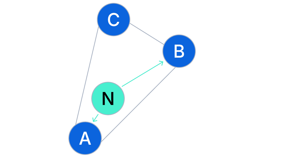
Node N is being added to the graph. New connections will be made from N to A and B, as the closest nodes, but not to C, as C is closer to B than it is to N. Then incoming connections to N are also made, from N’s newly connected neighbours back to N. These also take into account diversity, relative to the existing node, removing existing connections if that node’s connection limit has been reached to maintain diversity. These ensure that nodes are connected to a diverse selection of other nodes, maximising their reachability from elsewhere in the graph, and minimising the formation of fully-connected cliques.

But this does have a downside - because each node is not necessarily directly connected to all the nodes around it, a search for that node’s linked neighbours will not return complete results. This is one of the reasons approximate kNN search may miss some nodes that would be returned in an exhaustive search, and so reduce search recall compared with an exhaustive search, (see an example here).

Graph parameters

To summarize, the two parameters used to construct an HNSW graph are M (the maximum number of links a node can have) and ef_construction (how many nodes to search for neighbours when adding a new vector).

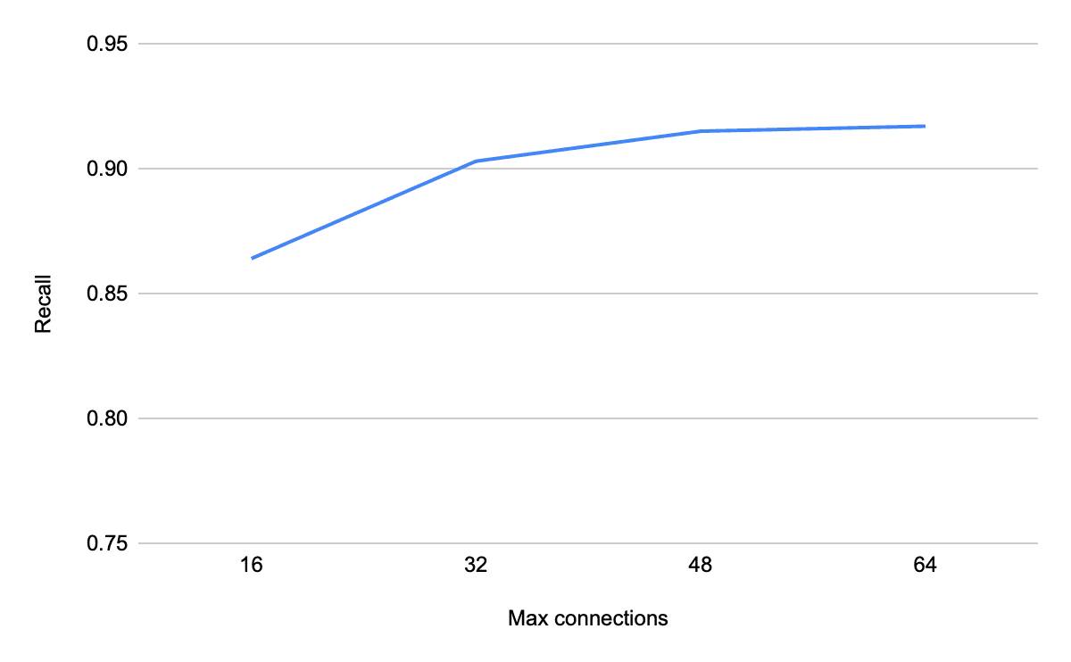
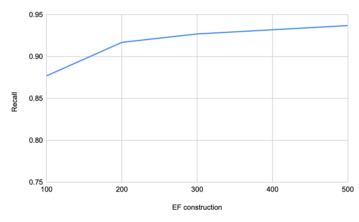
Increasing M makes searches more accurate by increasing the number of linked neighbours and the number of layers, but increases the disk and memory usage of the graph, the insertion latency, and the search latency.
Increasing ef_construction does a more exhaustive search to find neighbours for each new vector, but increases the insertion latency.

HNSW Graph FAQs:

These are the key points to understand the M and ef_construction graph construction parameters:

Question	Answer
What is an HNSW graph?	An HNSW (Hierarchical Navigable Small World) graph is a layered data structure for approximate nearest neighbor (ANN) search. All vectors are stored in the bottom layer, while upper layers contain fewer vectors that act as shortcuts, enabling faster traversal based on vector similarity.
How does an HNSW graph work?	An HNSW graph works by navigating layers top-down to locate the nearest neighbors. The search starts from an entry point in the highest layer, finds the closest vector, and uses it as the entry point for the next layer. This repeats until reaching the bottom layer, where a recursive search identifies the k nearest neighbors.
Why is an HNSW graph important?	HNSW graphs are important because they enable fast and scalable approximate nearest neighbor searches. The hierarchical structure allows efficient exploration of the vector space, reducing search time while preserving high recall.
How is an HNSW graph constructed?	An HNSW graph is constructed using two parameters: M (maximum connections per node) and ef_construction (neighbor search width). A new vector’s maximum layer is chosen randomly, then a search finds its nearest neighbors in each layer, and connections are established accordingly.
What is “diversity” in an HNSW graph?	Diversity in HNSW means the algorithm avoids cliques by enforcing connections to varied nodes. New connections are only made to nodes closer to the new vector than any existing neighbor, which improves reachability and prevents isolated clusters.